Univariate Derivatives

In this section, we introduce a visualization for computing derivatives of functions \(f: \mathbb{R} \to \mathbb{R}\). Not only will form the basis for both computing higher dimensional derivatives, but it will also get you in the habit of thinking graphically about functions. This will be especially useful when doing deep learning later.

Let us start nice and easy with basic functions over the reals as you have encountered them before, i.e. functions \(f: \mathbb{R} \to \mathbb{R}\). Though this initially may look superfluous, we will introduce a visual way of representing these functions. This new approach will make it easier to consider multivariate functions and is commonplace in machine learning. Consider the function \(f\) such that \(f: x \mapsto x^2\), i.e. the function that squares its input. Let \(y\) be the variable corresponding to the output of this function: \(y = f(x) = x^2\). We can visualize this function as follows:

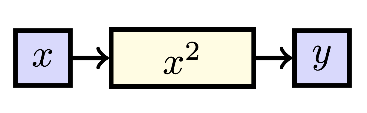
The blue squares represent values and the yellow rectangles represent ways to determine a value. The most important insight you should take away is that the sensitivity of \(y\) to \(x\) is given by the sum of influences of all the paths from \(x\) to \(y\). In this case, there is only one path, which is through the function \(x^2\). Using basic differentiation techniques, we hence observe that:

\[\frac{dy}{dx} = \frac{dx^2}{dx} = 2x.\]

A slightly more spicy example if the function \(f: \mathbb{R} \to \mathbb{R}\) such that \(f: x \mapsto \exp (\sin (x))\).¹ If we make a diagram of this function as above, we can represent it as follows:

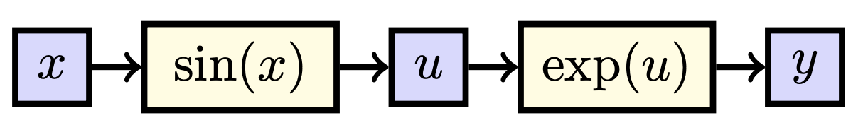
Please note that we had to introduce a new variable \(u:= \sin (x)\) that represents the intermediate value found after applying the sine function to \(x\). When finding the derivative of \(y\) with respect to \(x\), we again count all the paths from \(x\) to \(y\). Again, there is only one path, now going through our intermediate value \(u\). If we have a path with multiple variables on it, we multiply the intermediate effects. That is, the effect of \(x\) on \(y\) is equal to the effect of \(x\) on \(u\) times the effect of \(u\) on \(y\):

\[\frac{dy}{dx} = \frac{dy}{du} \frac{du}{dx}.\]

You may have encountered this separation of derivatives before as the chain rule. These derivatives are quite simple, giving us

\[\frac{dy}{dx} = \frac{dy}{du} \frac{du}{dx} = \exp(u) \cdot \cos (x) = \exp (\sin (x)) \cos (x),\]

where we substituted \(u = \sin (x)\) in the last step. So, we sum all the paths from \(x\) to \(y\), and we multiply the intermediate effects.

Let \(f: \mathbb{R} \to \mathbb{R}\) be the function defined by \(f: x \mapsto \sqrt{\tan (x^2)}\). Draw the diagram corresponding to this function and find \(\frac{df}{dx}\).

The corresponding diagram for this function is:

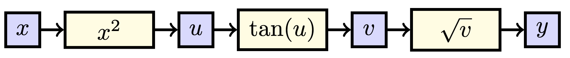
Here, we defined \(u := x^2\), \(v:= \tan u\), and \(y := \sqrt{v}\). The effect of \(x\) on \(f\) is given by the effect of \(x\) on \(u\) times the effect of \(u\) on \(v\) times the effect of \(v\) on \(y\), i.e.

\[\frac{df}{dx} = \frac{dy}{dv} \frac{dv}{du} \frac{du}{dx}.\]

Using basic derivative techniques, we, therefore, conclude that

\[\frac{df}{dx} = \frac{1}{2 \sqrt{v}} \cdot \frac{1}{\cos^2 u} \cdot 2 x.\]

Using our substitutions, we can write this as

\[\frac{df}{dx} = \frac{1}{2 \sqrt{\tan (x^2)}} \cdot \frac{1}{\cos^2 (x^2)} \cdot 2 x = \frac{x}{\cos^2(x^2) \sqrt{\tan (x^2)}}.\]

As you may remember, we know that when a derivative is equal to zero - i.e. when changing input \(x\) a bit has no effect on \(y\) - this must mean that we are in either a minimum or maximum of the function. This is why computing the derivative is so useful: it allows us to find these minima and maxima of functions, and if the function describes our model’s performance on a dataset given some parameters, the derivative will lead us to the parameter set that maximizes our model’s performance.

In this section, you have seen: a graphical visualization of functions and derivatives, the chain rule of differentiation, and the sum rule of differentiation in the context of standard functions \(f: \mathbb{R} \to \mathbb{R}\).