Multivariate Derivatives

Often - especially in machine learning - we are working with functions with multiple input and/or outputs. In this section, we study how our existing differentiation techniques extend to this multivariate case using our graphical representation as introduced in the previous section.

In general, we might be interested in functions with more than one input and output. For instance, if you give one input - e.g. a MRI scan - we might be interested in predicting a series of different outputs corresponding with different kinda of observations we could predict on the scan. Similarly, maybe we might want to predict the average time someone will spend in the coffee shop we opened based on their age, type of job, hobbies, and so on. In these cases, we would still like to compute derivatives of functions to estimate how well our model does, and in this case we have derivatives for each output with respect to each input.

Let’s go one step further, and consider a function \(f: \mathbb{R}^2 \to \mathbb{R}\) such that \(f: \begin{bmatrix}x_1 \\ x_2\end{bmatrix} \mapsto x_1x_2^2\). We can again draw this function:

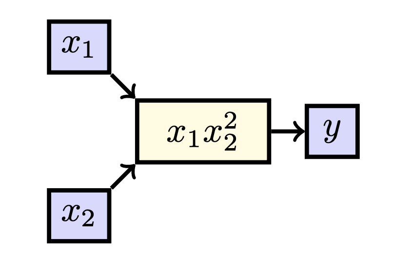
In this case, we can consider two derivatives: we can look at the effect of \(x_1\) on \(y\) and the effect of \(x_2\) on \(y\). When we can consider multiple derivatives for different variables, we do not write \(\frac{dy}{dx_1}\) but rather \(\frac{\partial y}{\partial x_1}\), to avoid confusion. We call such a derivative a partial derivative. Considering our earlier metaphor, a derivative of a standard real function is just the effect of turning a knob of a machine with one knob, whereas a partial derivative is an effect of turning one of the multiple knobs and keeping the other still. That is, \(\frac{\partial y}{\partial x_1}\) tells us how much \(y\) changes why \(x_1\) is increased while \(x_2\) is kept constant. As such, we can also treat \(x_2\) as a constant value when taking derivatives. Notice that as such we effectively have reduced the above setup to the uni-variate case.

In this case, we have that there is only one path from \(x_1\) to \(y\), and only one path from \(x_2\) to \(y\), giving us:

\[\frac{\partial y}{\partial x_1} = \frac{\partial x_1x_2^2}{\partial x_1} = x_2^2,\]

and

\[\frac{\partial y}{\partial x_2} = \frac{\partial x_1x_2^2}{\partial x_2} = 2x_1x_2.\]

What we sometimes do, is write the ‘full’ derivative \(\frac{d f}{d\textbf{x}}\) as the following vector:

\[\frac{dy}{d\textbf{x}} = \begin{bmatrix} \frac{\partial f}{\partial x_1} & \frac{\partial f}{\partial x_2} \end{bmatrix} = \begin{bmatrix}x_2^2 & 2x_1x_2\end{bmatrix},\]

where we understand \(\textbf{x} := \begin{bmatrix}x_1 \\ x_2 \end{bmatrix}.\)

We call this full derivative a gradient in the case we have functions \(f: \mathbb{R}^n \to \mathbb{R}\), denoted as \(\frac{dy}{d\textbf{x}} = \nabla y (\textbf{x}) = \text{grad } y(\textbf{x})\). However, in the the general case of functions \(f: \mathbb{R}^n \to \mathbb{R}^m\) we call the resulting matrix a Jacobian, denoted as \(\frac{d\textbf{y}}{d\textbf{x}} = \mathbf{J}_\textbf{y}(\textbf{x})\). The Jacobian is just the matrix which has on its \(i\) row all the partial derivatives of \(y_i\) with respect to \(x_j\), i.e. \(\mathbf{J}_{ij} = \frac{\partial y_i}{\partial x_j}\). Hence, since we only have one output here, we have that the Jacobian has only one row.¹

We can also have a function \(\textbf{f}: \mathbb{R} \to \mathbb{R}^2\) which maps \(\textbf{f}: x \mapsto \begin{bmatrix}x^2 \\ \sqrt{x} \end{bmatrix}.\) In this case, we have that \(\textbf{y} = \textbf{f}(x)\) where \(\textbf{y}\) is a vector (and hence is written in bold font), and thus we can consider \(y_1 = x^2\) and \(y_2 = \sqrt{x}\). Drawing this, we find:

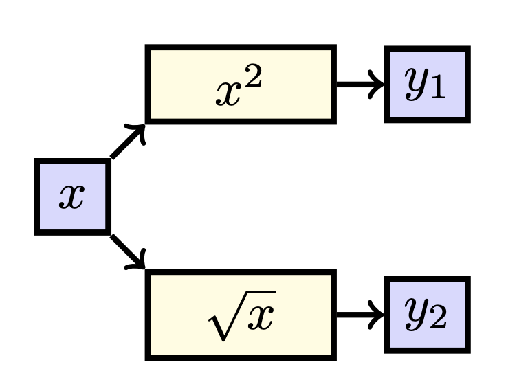
When again looking at the paths, we see that

\[\frac{d y_1}{dx} = \frac{d x^2}{dx} = 2x,\]

and

\[\frac{d y_2}{dx} = \frac{d \sqrt{x}}{dx} = \frac{1}{2\sqrt{x}}.\]

Here we can also group the different derivatives into one matrix:

\[\frac{d\textbf{y}}{dx} = \begin{bmatrix} 2x \\ \frac{1}{2\sqrt{x}} \end{bmatrix}.\]

Please note that if we have a function \(f: \mathbb{R}^n \to \mathbb{R}^m\) our Jacobian will be of the shape \(m \times n\).

Now we are finally ready to consider a function with multiple streams of influence. Consider the function \(f(x) = x^2 \ln (x).\) When breaking this functions into smaller parts, we can write is as \(y = g(\textbf{h}(x))\), where \(\textbf{h}(x) = (x^2, \ln (x))\) and \(g(u, v) = uv\). That is, \(y\) is found by first calculating intermediate values \(u = x^2\) and \(v = \ln (x)\) and then finding \(y= uv.\) If we draw these functions, we see the following:

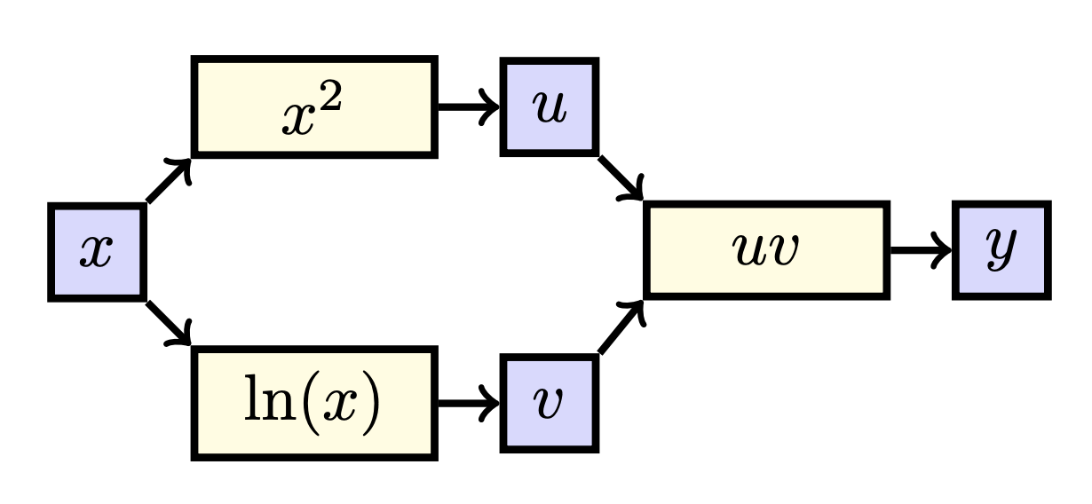
It is now very clear that the effect of \(x\) of \(y\) is twofold: both through \(u\) and \(v\). As mentioned earlier, we need to consider all streams of influence. Specifically, we sum the different paths/effects, i.e.:

\[\frac{d y}{dx} = \frac{\partial y}{\partial u} \frac{du}{dx} + \frac{\partial y}{\partial v} \frac{dv}{dx}.\]

Plugging everything in, we find

\[\frac{d y}{dx} = \frac{\partial y}{\partial u} \frac{du}{dx} + \frac{\partial y}{\partial v} \frac{dv}{dx} = v \cdot 2x + u \cdot \frac{1}{x} = \ln(x) \cdot 2x + x^2 \cdot \frac{1}{x} = 2x (\ln (x) + \frac{1}{2}).\]

You may recognize this as the product rule, now you know where that comes from!

Suppose \(\textbf{f}: \mathbb{R}^3 \to \mathbb{R}^3\) such that \(f(x_1, x_2, x_3) = \textbf{h}(\textbf{g}(x_1, x_2, x_3))\), where \(\textbf{g}(x_1, x_2, x_3) = (x_1^2x_2^2, \sqrt{x_2x_3})\) and \(\textbf{h}(u, v) = (u^2, uv, v^2)\). Find \(\frac{\partial y_2}{\partial x_2}\). Hint: draw out what happens.

When visualizing this function, we get the following:

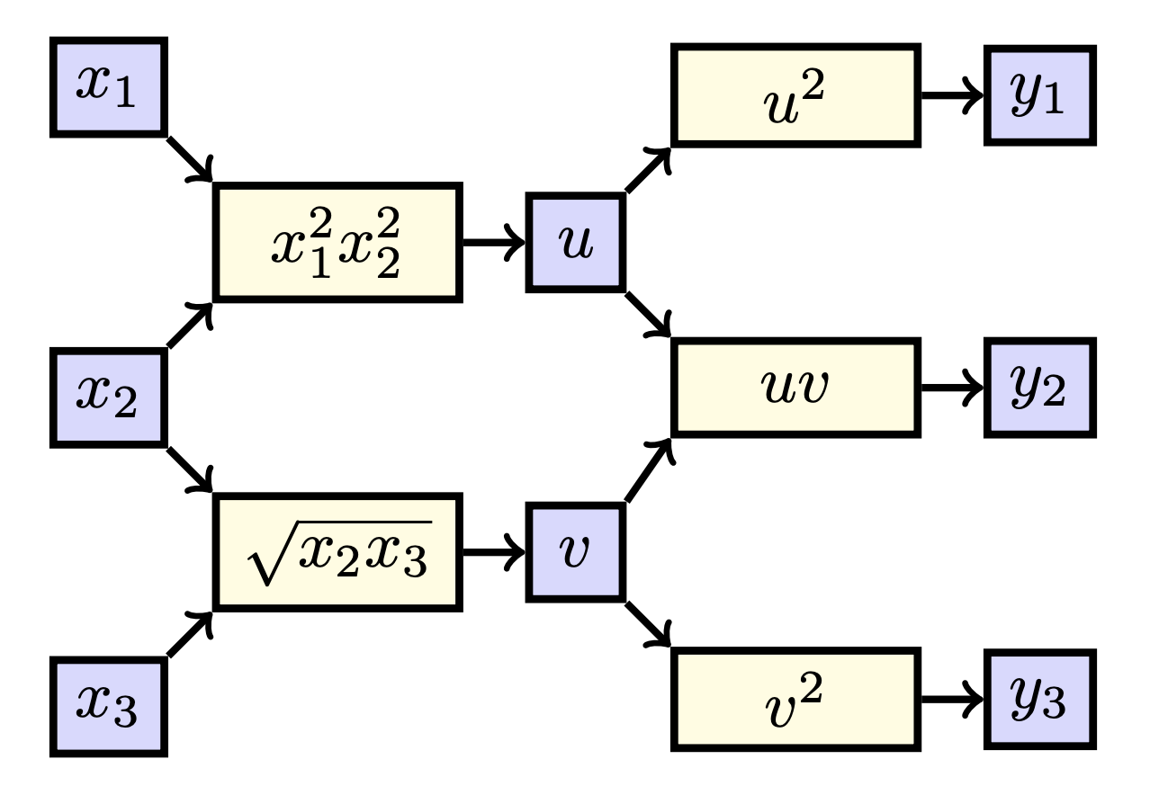
When counting the paths from \(x_2\) to \(y_2\), we find two paths: one through \(u\) and one through \(v\). We hence find

\[\frac{\partial y_2}{\partial x_2} = \frac{\partial y_2}{\partial u} \frac{\partial u}{\partial x_2} + \frac{\partial y_2}{\partial v} \frac{\partial v}{\partial x_2}.\]

Plugging our derivatives, we find

\[\frac{\partial y_2}{\partial x_2} = v \cdot 2x_1^2x_2 + u \cdot \frac{x_3}{2\sqrt{x_2x_3}} = 2x_1^2 x_2 \sqrt{x_2x_3} + \frac{x_1^2 x_2^2x_3}{2\sqrt{x_2x_3}}.\]

Sweet! We now know how to find derivatives in multivariate functions. As you have seen, this approach is quite a time intensive, and sometimes (especially in deep learning) it is not necessary to write out everything by hand like this. This will be the topic of the rest of this section.

In this section we extended our graphical interpretation of derivatives to functions \(f: \mathbb{R}^m \to \mathbb{R}^n\).